Show code cell source Hide code cell source

import numpy as np
import pandas as pd
import matplotlib.pyplot as plt
import seaborn as sns
from sklearn.preprocessing import StandardScaler, MinMaxScaler
from sklearn.model_selection import train_test_split
from sklearn.linear_model import LinearRegression

from rdkit import Chem
from rdkit.Chem import (
                        PandasTools,
                        Descriptors
                        )

from rdkit.Chem.Draw import IPythonConsole

Notebook - ML for thermochemical data prediction

We can use the data you worked with for the EDA workshop to demonstrate how fit a simple ML model to predict the boiling point of organic compounds from a small set of descriptors.

This is an example of

Supervised learning as applied to a regression task.

Supervised learning

The model learns from data for which a label (known value or category) is associated with each input (set of feature values)

Regression task

Model predicts a continuous numerical value based on the input features

bp_df = pd.read_csv("data/alcohol_acid_phys_data_cleaned.csv")
bp_df

	Class	IUPAC name	#C	#H	#O	Molweight g/mol	mp / dC	bp / dC	density / g/ml	SMILES
0	1-alkanol	Methanol	1	4	1	32.04	-98.0	65	0.7910	CO
1	1-alkanol	Ethanol	2	6	1	46.07	-114.0	78	0.7890	CCO
2	1-alkanol	1-Propanol	3	8	1	60.09	-124.0	97	0.8040	CCCO
3	1-alkanol	1-Butanol	4	10	1	74.12	-89.0	118	0.8100	CCCCO
4	1-alkanol	1-Pentanol	5	12	1	88.15	-78.0	138	0.8140	CCCCCO
...	...	...	...	...	...	...	...	...	...	...
73	Branched alkanoic acid	4-Methylpentanoic acid	6	12	2	116.16	-33.0	200	0.9230	CC(C)CCC(O)=O
74	Benzoic acids	Benzoic acid	7	6	2	122.12	122.0	249	1.2660	OC(=O)c1ccccc1
75	Benzoic acids	2-Methyl-benzoic acid	8	8	2	136.14	107.0	258	1.0620	Cc1ccccc1C(O)=O
76	Phenyl- alkanoic acid	Phenylethanoic acid	8	8	2	136.14	77.0	266	1.2286	OC(=O)Cc1ccccc1
77	Alkanedioic acid	Decanedioic acid	10	18	4	202.24	131.0	374	1.2710	OC(=O)CCCCCCCCC(O)=O

78 rows × 10 columns

The data is read in from a csv file of the data cleaned in the EDA workshop, so should be prepared, but we can quickly check.

# Check for missing values
bp_df.isna().sum()

Class              0
IUPAC name         0
#C                 0
#H                 0
#O                 0
Molweight g/mol    0
mp / dC            0
bp / dC            0
density / g/ml     0
SMILES             0
dtype: int64

# Check data types
bp_df.info()

<class 'pandas.core.frame.DataFrame'>
RangeIndex: 78 entries, 0 to 77
Data columns (total 10 columns):
 #   Column           Non-Null Count  Dtype  
---  ------           --------------  -----  
 0   Class            78 non-null     object 
 1   IUPAC name       78 non-null     object 
 2   #C               78 non-null     int64  
 3   #H               78 non-null     int64  
 4   #O               78 non-null     int64  
 5   Molweight g/mol  78 non-null     float64
 6   mp / dC          78 non-null     float64
 7   bp / dC          78 non-null     int64  
 8   density / g/ml   78 non-null     float64
 9   SMILES           78 non-null     object 
dtypes: float64(3), int64(4), object(3)
memory usage: 6.2+ KB

The numerical types are as expected. The category type for the class column has not been automatically recognised, understandably. For now we will not be working with that column, so will leave as is.

We will start by dropping any rows without a SMILES string and also the melting point column as we are going to try to predict the boiling point.

# Drop rows with missing SMILES string
bp_df = bp_df[bp_df["SMILES"] != "not found"].reset_index(drop=True)

bp_df = bp_df.drop(columns=["mp / dC"])
bp_df

	Class	IUPAC name	#C	#H	#O	Molweight g/mol	bp / dC	density / g/ml	SMILES
0	1-alkanol	Methanol	1	4	1	32.04	65	0.7910	CO
1	1-alkanol	Ethanol	2	6	1	46.07	78	0.7890	CCO
2	1-alkanol	1-Propanol	3	8	1	60.09	97	0.8040	CCCO
3	1-alkanol	1-Butanol	4	10	1	74.12	118	0.8100	CCCCO
4	1-alkanol	1-Pentanol	5	12	1	88.15	138	0.8140	CCCCCO
...	...	...	...	...	...	...	...	...	...
72	Branched alkanoic acid	4-Methylpentanoic acid	6	12	2	116.16	200	0.9230	CC(C)CCC(O)=O
73	Benzoic acids	Benzoic acid	7	6	2	122.12	249	1.2660	OC(=O)c1ccccc1
74	Benzoic acids	2-Methyl-benzoic acid	8	8	2	136.14	258	1.0620	Cc1ccccc1C(O)=O
75	Phenyl- alkanoic acid	Phenylethanoic acid	8	8	2	136.14	266	1.2286	OC(=O)Cc1ccccc1
76	Alkanedioic acid	Decanedioic acid	10	18	4	202.24	374	1.2710	OC(=O)CCCCCCCCC(O)=O

77 rows × 9 columns

# Add RDKit molecules to the dataframe
PandasTools.AddMoleculeColumnToFrame(bp_df, smilesCol="SMILES")
bp_df

	Class	IUPAC name	#C	#H	#O	Molweight g/mol	bp / dC	density / g/ml	SMILES	ROMol
0	1-alkanol	Methanol	1	4	1	32.04	65	0.7910	CO
1	1-alkanol	Ethanol	2	6	1	46.07	78	0.7890	CCO
2	1-alkanol	1-Propanol	3	8	1	60.09	97	0.8040	CCCO
3	1-alkanol	1-Butanol	4	10	1	74.12	118	0.8100	CCCCO
4	1-alkanol	1-Pentanol	5	12	1	88.15	138	0.8140	CCCCCO
...	...	...	...	...	...	...	...	...	...	...
72	Branched alkanoic acid	4-Methylpentanoic acid	6	12	2	116.16	200	0.9230	CC(C)CCC(O)=O
73	Benzoic acids	Benzoic acid	7	6	2	122.12	249	1.2660	OC(=O)c1ccccc1
74	Benzoic acids	2-Methyl-benzoic acid	8	8	2	136.14	258	1.0620	Cc1ccccc1C(O)=O
75	Phenyl- alkanoic acid	Phenylethanoic acid	8	8	2	136.14	266	1.2286	OC(=O)Cc1ccccc1
76	Alkanedioic acid	Decanedioic acid	10	18	4	202.24	374	1.2710	OC(=O)CCCCCCCCC(O)=O

77 rows × 10 columns

Show code cell source Hide code cell source

# Adapted from https://greglandrum.github.io/rdkit-blog/posts/2022-12-23-descriptor-tutorial.html

def getMolDescriptors(mol, descriptor_list=None, missingVal=None):
    ''' calculate the full list of descriptors for a molecule
    
        missingVal is used if the descriptor cannot be calculated
    '''
    res = {}
    if not(descriptor_list):
        descriptors = Descriptors._descList
    # TODO: Add else clause to handle a list numbers corresponding to the descriptor indices
    else:
        descriptors = [Descriptors._descList[idx] for idx in descriptor_list]

    for nm,fn in descriptors:
        # some of the descriptor fucntions can throw errors if they fail, catch those here:
        try:
            val = fn(mol)
        except:
            # print the error message:
            import traceback
            traceback.print_exc()
            # and set the descriptor value to whatever missingVal is
            val = missingVal
        res[nm] = val
    return res

# These are the descriptors selected to calculate for the molecules.
# 118 NumHAcceptors
# 119 NumHDonors
# 27 BalabanJ - a topological descriptor expressing molecular connectivity and branching
# 28 BertzCT - a topological complexity index
# 83 TPSA - total polar surface area

descriptor_list = [118, 119, 27, 28, 83]


calc_descriptors = [getMolDescriptors(mol, descriptor_list=descriptor_list) for mol in bp_df["ROMol"]]

# Create a dataframe from the calculated descriptors
descriptor_df = pd.DataFrame(calc_descriptors)

# Add the descriptors to the dataframe as new columns
bp_df = pd.concat([bp_df, descriptor_df], axis=1)
bp_df

	Class	IUPAC name	#C	#H	#O	Molweight g/mol	bp / dC	density / g/ml	SMILES	ROMol	NumHAcceptors	NumHDonors	BalabanJ	BertzCT	TPSA
0	1-alkanol	Methanol	1	4	1	32.04	65	0.7910	CO	<rdkit.Chem.rdchem.Mol object at 0x154fd8c10>	1	1	1.000000	2.000000	20.23
1	1-alkanol	Ethanol	2	6	1	46.07	78	0.7890	CCO	<rdkit.Chem.rdchem.Mol object at 0x154fd8eb0>	1	1	1.632993	2.754888	20.23
2	1-alkanol	1-Propanol	3	8	1	60.09	97	0.8040	CCCO	<rdkit.Chem.rdchem.Mol object at 0x154fd8f90>	1	1	1.974745	5.245112	20.23
3	1-alkanol	1-Butanol	4	10	1	74.12	118	0.8100	CCCCO	<rdkit.Chem.rdchem.Mol object at 0x154fd8f20>	1	1	2.190610	11.119415	20.23
4	1-alkanol	1-Pentanol	5	12	1	88.15	138	0.8140	CCCCCO	<rdkit.Chem.rdchem.Mol object at 0x154fd9000>	1	1	2.339092	15.900135	20.23
...	...	...	...	...	...	...	...	...	...	...	...	...	...	...	...
72	Branched alkanoic acid	4-Methylpentanoic acid	6	12	2	116.16	200	0.9230	CC(C)CCC(O)=O	<rdkit.Chem.rdchem.Mol object at 0x154fdaea0>	1	1	3.050078	76.597721	37.30
73	Benzoic acids	Benzoic acid	7	6	2	122.12	249	1.2660	OC(=O)c1ccccc1	<rdkit.Chem.rdchem.Mol object at 0x154fdaf10>	1	1	2.981455	203.415953	37.30
74	Benzoic acids	2-Methyl-benzoic acid	8	8	2	136.14	258	1.0620	Cc1ccccc1C(O)=O	<rdkit.Chem.rdchem.Mol object at 0x154fdaf80>	1	1	3.152941	253.189433	37.30
75	Phenyl- alkanoic acid	Phenylethanoic acid	8	8	2	136.14	266	1.2286	OC(=O)Cc1ccccc1	<rdkit.Chem.rdchem.Mol object at 0x154fdaff0>	1	1	2.674242	215.959017	37.30
76	Alkanedioic acid	Decanedioic acid	10	18	4	202.24	374	1.2710	OC(=O)CCCCCCCCC(O)=O	<rdkit.Chem.rdchem.Mol object at 0x154fdb060>	2	2	2.989544	156.960812	74.60

77 rows × 15 columns

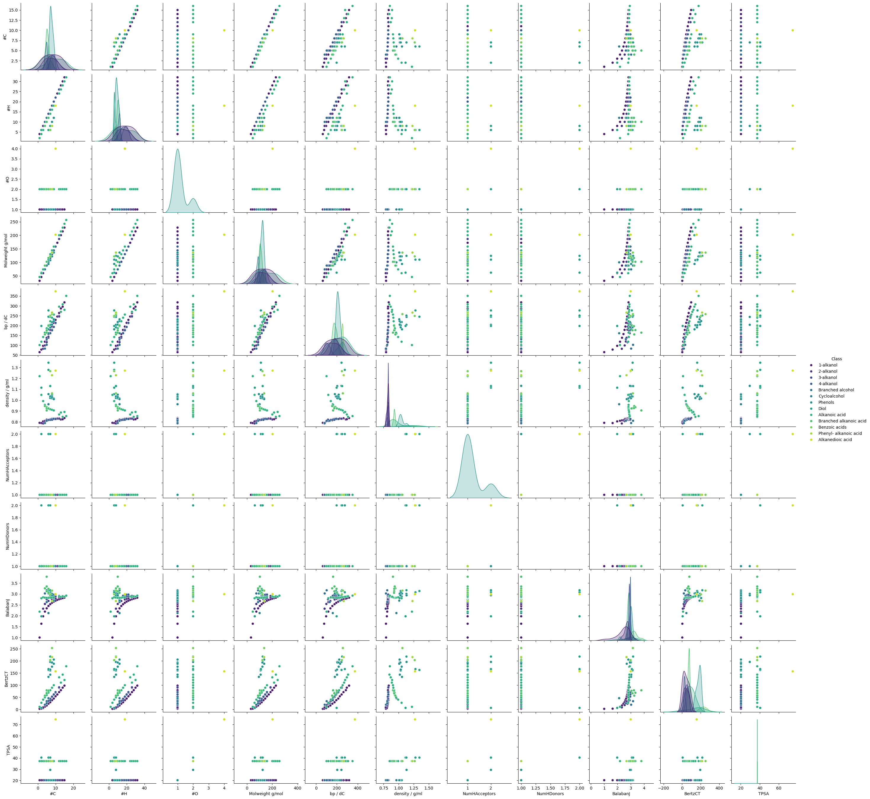
# To remind us of the relationship between the variables, we can plot a pairplot and heatmap
# Pairplot
sns.pairplot(bp_df, hue="Class", diag_kind="kde",  palette="viridis")
plt.show()

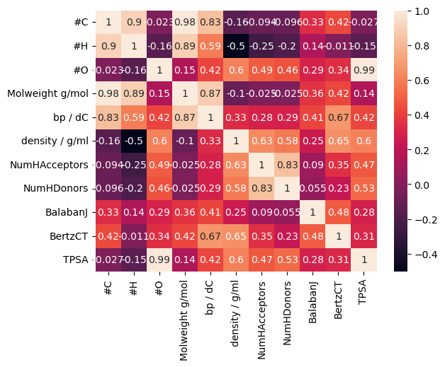
corr = bp_df.drop(columns=["Class", "IUPAC name", "SMILES", "ROMol"]).corr()

sns.heatmap(corr, annot=True)
plt.show()

# corr_abs = bp_df.drop(columns=["Class", "IUPAC name", "SMILES", "ROMol"]).corr().abs()
# upper = corr_abs.where(np.triu(np.ones(corr.shape), k=1).astype(bool))
# upper

This is all looking rather busy - it would be better to look at subsets of the features.

What we can see is:

• The feature most strongly correlated with the target variable is the molecular weight.

• Molecular weight is very strongly correlated with number of carbons and hydrogens

• Most of the other features are only moderately or weakly correlated to the target variable.

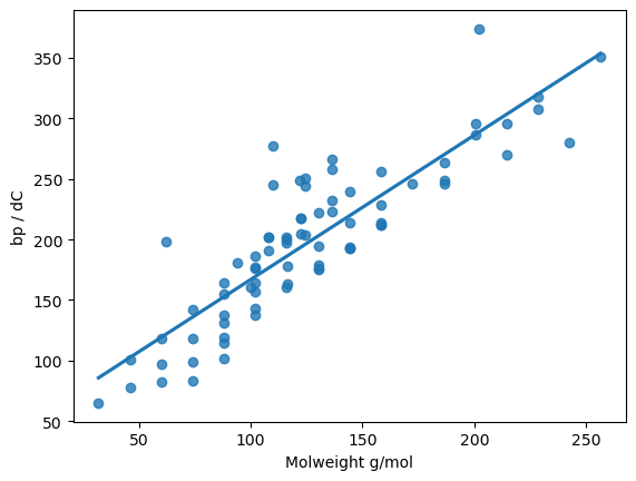
# A closer look at the correlation between the boiling point and the molecular weight
sns.regplot(data=bp_df, x="Molweight g/mol", y="bp / dC",  fit_reg=True,  ci=None)
plt.show()

For the moment, we will drop the #C and #H columns. We will see that analysing the initial model can help tell us about the importance of the features.

We will also drop the non-numerical features for this task.

cols_drop = ["#C", "#H", "IUPAC name", "SMILES", "ROMol", "Class"]

prep_df = bp_df.drop(columns=cols_drop)
prep_df

	#O	Molweight g/mol	bp / dC	density / g/ml	NumHAcceptors	NumHDonors	BalabanJ	BertzCT	TPSA
0	1	32.04	65	0.7910	1	1	1.000000	2.000000	20.23
1	1	46.07	78	0.7890	1	1	1.632993	2.754888	20.23
2	1	60.09	97	0.8040	1	1	1.974745	5.245112	20.23
3	1	74.12	118	0.8100	1	1	2.190610	11.119415	20.23
4	1	88.15	138	0.8140	1	1	2.339092	15.900135	20.23
...	...	...	...	...	...	...	...	...	...
72	2	116.16	200	0.9230	1	1	3.050078	76.597721	37.30
73	2	122.12	249	1.2660	1	1	2.981455	203.415953	37.30
74	2	136.14	258	1.0620	1	1	3.152941	253.189433	37.30
75	2	136.14	266	1.2286	1	1	2.674242	215.959017	37.30
76	4	202.24	374	1.2710	2	2	2.989544	156.960812	74.60

77 rows × 9 columns

from sklearn.model_selection import train_test_split
from sklearn.preprocessing import MinMaxScaler

# By convention, the target variable is denoted by y and the features are denoted by X

y_full = prep_df["bp / dC"]
X_full = prep_df.drop(columns=["bp / dC"])

# train_test_split shuffles the data by default and splits it into training and testing sets. The 
# proportion of the data that is used for testing is determined by the test_size parameter. Here, 
# we are using 80 % of the data for training and 20% for the test set. 
# The random_state parameter is used to set the seed for the random number generator so that the 
# results are reproducible.

X_train, X_test, y_train, y_test = train_test_split(X_full, y_full, test_size=0.2, random_state=42)

# Check the size of the training and testing sets
X_train.shape, X_test.shape, y_train.shape, y_test.shape

((61, 8), (16, 8), (61,), (16,))

Scikit-learn makes many models available via a consistent interface.

We are going to use a linear regression model for this task.

from sklearn import linear_model

# Create a linear regression model
reg = linear_model.LinearRegression()

# Fit the model to the training data
reg.fit(X_train, y_train)

LinearRegression()

In a Jupyter environment, please rerun this cell to show the HTML representation or trust the notebook.
On GitHub, the HTML representation is unable to render, please try loading this page with nbviewer.org.

# Predict the boiling points of the test set
y_pred = reg.predict(X_test)

We can plot the boiling points that the model predicted for the test set against the known true values to see how good a job the model makes of the predictions

plt.scatter(y_test, y_pred)
plt.plot([y_test.min(), y_test.max()], [y_test.min(), y_test.max()], '-', lw=1, color="red")
plt.xlabel("True Values [bp / dC]")
plt.ylabel("Predictions [bp / dC]")
plt.show()

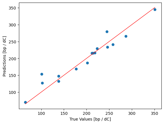
# The r^2 value is a measure of how well the model fits the data. It ranges from 0 to 1, 
# with 1 indicating a perfect fit.
r2 = reg.score(X_test, y_test)
r2

0.9287935935680889

If we look back, we can see that the Pearson correlation coefficient for the relationship between molecular weight and boiling point was 0.84, so the model predicts more accurately than using the molecular weight alone.

The model coefficients tell us about the weighting of the features used by the fitted model.

print(X_full.columns)
reg.coef_

Index(['#O', 'Molweight g/mol', 'density / g/ml', 'NumHAcceptors',
       'NumHDonors', 'BalabanJ', 'BertzCT', 'TPSA'],
      dtype='object')

array([-1.76222475e+01,  1.17239618e+00,  1.64551206e+02, -2.42988355e+00,
        2.57293551e+01, -6.34194132e+00,  5.78435772e-02,  1.26142804e+00])

However, because the magnitude of the features’ values are on different scales, the coefficients also incorporate the different scales.

A scaler can be used to transform the features to a consistent scale. Here’s we’ll use a MinMaxScaler to transform the features to have a scale between 0 and 1.

# Split the scaled data into training and testing sets
X_train, X_test, y_train, y_test = train_test_split(X_full, y_full, test_size=0.2, random_state=42)

# create a min/max scaler
scaler = MinMaxScaler()

# fit the scaler to the training data
scaler.fit(X_train)

# transform the training and testing data separately
scaled_X_train = scaler.transform(X_train)
scaled_X_test = scaler.transform(X_test)

# Create a linear regression model
reg = linear_model.LinearRegression()

# Fit the model to the training data
reg.fit(scaled_X_train, y_train)

# Predict the boiling points of the test set
y_pred = reg.predict(scaled_X_test)

plt.scatter(y_test, y_pred)
plt.plot([y_test.min(), y_test.max()], [y_test.min(), y_test.max()], '-', lw=1, color="red")
plt.xlabel("True Values [bp / dC]")
plt.ylabel("Predictions [bp / dC]")
plt.show()

# calculate the R^2 score
r2 = reg.score(scaled_X_test, y_test)
r2

0.9287935935680927

The model’s predictions look the same as before, but we can now look at the coefficients.

print(X_full.columns)
reg.coef_

Index(['#O', 'Molweight g/mol', 'density / g/ml', 'NumHAcceptors',
       'NumHDonors', 'BalabanJ', 'BertzCT', 'TPSA'],
      dtype='object')

array([  1.65984399, 230.16481816,  81.1237445 , -10.77763669,
        37.44176379, -13.68670374,  12.45958115,  10.69260041])

We can now see that the coefficients which represent the weights of the features in the fitted model indicate that molecular weight - as expected - and density are contributing most strongly to the model